

Sometimes inventory is a pure pass-through, such as for typical trade businesses. Sometimes it is developed and transformed via work conducted within the firm into a final product, such as for typical producing businesses. And sometimes it simply transforms itself into the final product – without any meaningful contribution of the company. This latter case is a quite interesting one from a financial analysis point of view because it has some effects which differ from our typical accounting understanding. This is why it is worth to shed some more light on it here.
Self-transforming inventory itself can be split into two versions. The first one has already been discussed in this blog (LINK). It is about IAS 41 Agriculture. This standard covers the accounting treatment for so called biological assets. These are assets which are to be sold at a later point in time via the normal revenue generating process of the company and which are somehow in a living state. This could be animals (like salmons in a salmon farm) or living plant (like typical agricultural assets). The standard generally requires such assets to be measured at fair value less costs to sell. As a matter of course this accounting treatment is a tricky one as it requires an often at least softly-subjective assessment on fair values of such inventory-assets without any clear market indication for them. But today we rather want to look at the other version.
This second version is about similarly characterised inventory which, however, does not fall under the category of biological assets (although the fundamental difference is quite small). This could be e.g. some sort of art, wine or – as in our case – liquor. Diageo plc. is a UK-based international alcoholic beverages company, one of the world’s largest distiller and runs amongst others brands such as Johnnie Walker (Whiskey), Don Julio (Tequila) or Captain Morgan (Rum) but also many other famous liquor products. Many of these liquor products cannot be sold shortly after production (distillation) but require a maturation stage which makes them to the product that customers want to buy, e.g. for some whiskeys not rarely much more than ten years, for others only two or three years. You can see the similarity to the IAS 41 biological assets here, but for some reasons Diageo’s ageing liquor products do not fall under this standard. They are rather accounted for according to the normal ‘lower of cost or market” inventory accounting principles of IAS 2. Of course there are some differences between typical IAS 41 inventories which usually cannot be sold to the end-customer before reaching maturity and liquors which often could be sold before but will not find the price or attractiveness that typical customers require or a seeking for. But the economic differences are quite small in reality. Anyway, Diageo has to account for its ageing liquors according to IAS 2.
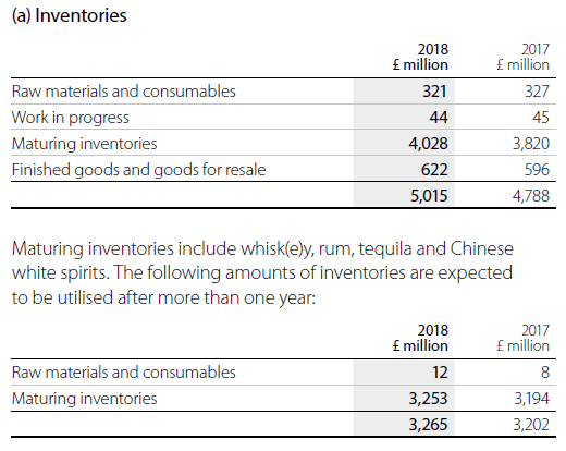
Let’s first have a look at how Diageo’s maturing liquor business developed over time.
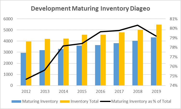
Source: Diageo Annual Reports (ARs), absolute numbers in mio GBP, financial year end: June.
Obviously, Diageo has increased its maturing inventory business over the last years, both in absolute as well as in relative terms.
For better understanding what this means for financial analysis it is now first necessary to have a general look at the financial consequences of selling such maturing inventory which does not fall under IAS 41. In a normal business environment where these inventories gain in value (financial, not accounting) over time we would see a higher gross margin in the accounts as compared to a company which sells non-maturing inventory. This is simply the case as the costs of goods sold are fuelled with the accounting inventory value which is usually at original ‘cost’. The price-to-be-paid for this higher gross margin is that during the build-up phase of such businesses the revenues and the gross profit lags comparable companies which do not sell maturing inventories (simply because the company cannot sell anything until the inventory is matured) and by a higher inventory stock even in a steady state as the company always carries some maturing inventories which are not yet ready to be sold.
We show this by a hypothetical (and simplified) example of two companies – Company (1) which sells the inventory it bought at the beginning of the period at the end of the same period, and Company (2) which waits for maturation of inventory for three periods and sells the inventory at the end of this period t+3.
It is further assumed that the maturing inventory gains in (fair market, not accounting) value every period exactly by 10% (which is also the cost of capital of both companies) and that both companies are able to sell the inventory at a price 10% higher than beginning of period value. These assumptions help us to isolate the different financial, value and accounting impacts.
Furthermore, in our simplified example there are no other costs to the company, no interest payments (they are all-equity financed) and no taxes. Furthermore, we only look at a no-growth scenario.
The table below shows the first 8 periods of Company (1).
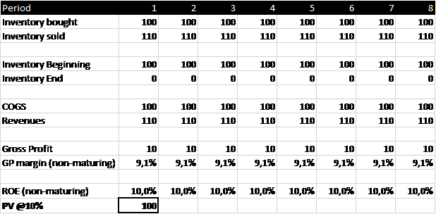
We think the numbers are not a big surprise. ROE is calculated here in accounting terms, i.e. by dividing gross profit for the period by beginning of period capital (inventory). The present value (beginning of period 1) is calculated by discounting future cash flows – which here equal the gross profits – at the cost of capital of 10% until eternity.
Now let’s have a look at the same table for Company (2).
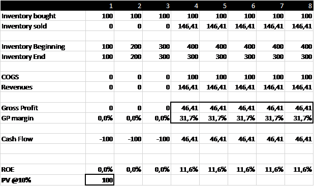
Company (2) here starts with this business from scratch in period 1. During the first three periods they do not generate any revenues because inventory is still in a maturing state. Due to the periodization principle of accounting during these periods (costs of input products only show up as expenses in the period they are sold) no COGS are recorded, neither. Then starting in period 4, revenues are recorded. The respective COGS relate to the inventory at ‘cost’ (or better: at lower of cost or market – which is ‘cost’ here). Due to the fair value increase of inventory Company (2) can now generate much higher gross profits and gross margins than the comparable Company (1). Interestingly, the period 0 present value of both strategies is the same – this is because our assumptions are that the fair value of maturing inventory increases exactly at the cost of capital over time.
Comment 1: Once Company (2) has reached the steady state in period 4, however, its present value seems to be higher than that of the comparable company (1). This is the case here as now the negative cash flow periods 1-3 (where Company (2) spend money for building up inventory without generating revenues) are behind us. But this finding is also only due to the simplified nature of our example. We do not look at the question of how Company (2) covers the period 1-3 negative cash flows. Perhaps it does so via debt issuance (in our simplified example probably via equity issuance or use of the cash position as the cost of capital do not change over time). In reality it might well be that there is a net-zero or even net-negative effect of this strategy once entering into the stead state – but this is out of the scope of our analysis here. In a normal business environment – with no outperformance of fair value increases of maturing inventory vis-á-vis the cost of capital – the net-PV-effect of this strategy is always zero. So we cannot make hard statements on PV development, but we can definitely say that the gross profits and gross margins are higher for Company (2).
Comment 2: As we are looking at a no growth state without any inflationary effects it does not matter here which IFRS inventory valuation principle the company follows (FIFO or weighted average costs). In reality (i.e. an environment with price changes over time for input products) these numbers might, however, differ a bit from the clear-cut analysis above.
Comment 3: Accounting ROEs are higher here as compared to the Company (1) case. This is just an accounting issue as the periodical cash flow effects (input vs. output) go astray. This is an extremely important issue in general with regards to performance measurement but not the focus of this analysis here. If you want to know more about this general problem of financial analysis, wait for some later posts here in this blog or have a look at a recently published academic article by Felix Streitferdt, Max Levasier and me HERE.
This comparison of Company (1) and Company (2) is important for at least three reasons.
First, one of the most important finding in terms of factor investing in recent years was the analysis of Robert Novy-Marx on the “Gross Profitability Premium” (Novy-Marx, 2013, The Other Side of Value: The Gross Profitability Premium, in: Journal of Financial Economics, Vol. 108 (1), p. 1-28). He detected a systematic valuation premium for high gross-profit firms in the cross-section of average returns, at a similar size to the book-to-market premium of the famous Fama/French analyses. The most-plausible explanation for this finding is that companies with a relatively high gross profit have a high pricing power, i.e. for several reasons (strong brand, reputation, quality of products, etc.) they are able to sell their products at a relatively higher price than competitors, and this advantage translates into a strong and enduring competitive positioning. This is not new in terms of how value investors try to isolate high-quality companies but it has never before been formalized like this. Today quant investors as well as fundamental investors certainly look closer at the gross margins of companies than they did before Novy-Marx’ analysis.
However, The gross margin of companies which run a maturing inventory business – such as Diageo – is not necessarily a function of pricing power (in the case of Diageo: for some liquors: yes, for some others: no). It is mainly simply a function of the maturing inventory business per se and its accounting treatment, as was shown in our hypothetical example above. So investors might get trapped by misunderstanding Diageo’s assumably increasing gross margin because it has nothing to do per se with pricing power but rather with the nature of the business and the accounting which could not map this business properly.
Second, the real interesting case is when companies more or less slowly build up their maturing inventory business over time (as Diageo does it currently according to our analyses above but they have certainly already reached the kick-in phase). This strategy is not totally different from other build-up strategies that we have already discussed in this blog, e.g. the three-is-a-crowd strategy in the context of reverse factoring, see LINK .
To highlight the effects of this strategy we adjust our hypothetical example a bit. We now combine Company (1) and Company (2) in one case by simply assuming that the original Company (1) starts to substitute non-maturing inventory by maturing inventory step-by-step over time – here in periodical steps of 5 Euros out of the original 100 Euro investment in inventory. The total amount of how much inventory is bought stays constant over time (i.e. the sum of inventory bought maturing and inventory bought non-maturing remains at 100). Here is the new table.
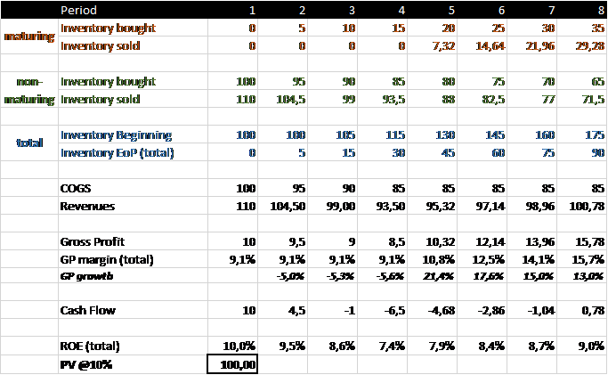
Now, we can see some interesting patterns. Of course, during the first three periods of change the company records a negative gross profit growth but once the maturing inventory sales kick-in this changes to a positive growth (as the company now starts to approach the higher Company (2) gross profit level step-by-step). The gross margin does not suffer in the first three periods due to periodization rules of accounting. Cash flows, however, show a lagged effects (the company has to invest [cash-out] in order to realise the switch) due to the step-wise change to higher pronunciation of maturing inventory over time. And finally, the present value – here calculated over more than the here shown 8 periods but rather over the total life of this strategy – of this company’s equity is still at 100 Euros at the beginning (and as mentioned above: in an environment of financing requirements of negative cash flows and hence increasing net debt it would also not differ from the PV patterns over time from the above examples as long as fair value increases are exactly at the cost of capital).
And one important last point: inventory – and hence capital tie-up – increases over time.
Things get even clearer if we have a look at more than these 8 periods. Here is the picture for the whole strategy until period 30 where the company switches to a maturing-inventory-only business (this translation lasts full non-maturing inventory business exposure is reached in period 21).
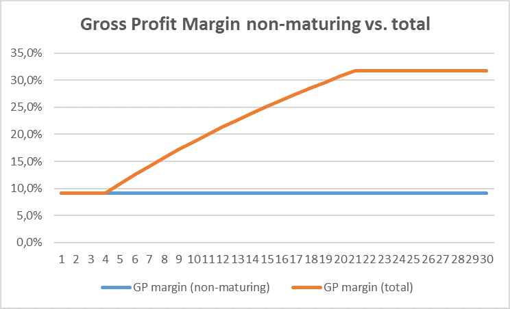
We can nicely see here how the gross profit margin increases over time.
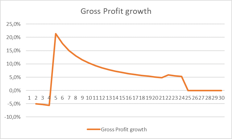
Accordingly, we can also see that the growth of gross profit is highly positive starting with the kick-in of the maturing inventory and until the strategy is fully implemented (i.e. at 100% maturing inventory only). The strange pattern of the growth functional starting in period 22 is due to the expiry of the non-maturing inventory sales – just an accounting effect here.
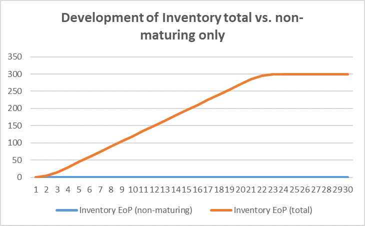
We can also see the capital tie-up that increases over time by focussing more and more on maturing inventory (EoP: End of Period). For reasons of comparison we have mapped the inventory development of non-maturing inventory only: No surprise, it stays at zero over time as these input products are immediately sold in this period. This will become important later in our analysis.
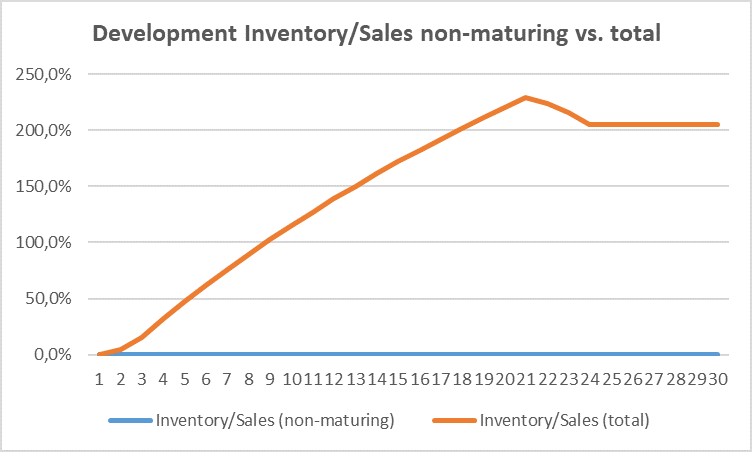
Accordingly, we can also show the development of inventory divided by sales over time.
And finally the returns on equity over time:
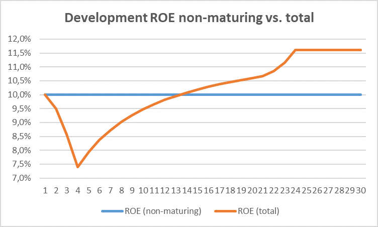
Again, we have included the original Company (1) case as a comparison. You can see here the weak start in accounting ROE performance at the beginning of the switching strategy and then the gradual increase to the higher Company (2) number over time.
As an interim summary: With this switching strategy companies can generate profit growth even at a constant level of investments over time and without any additional capex – once the maturing inventory sales kick-in. This growth, however, is just a result of the transformation of one business model to the other. The growth is fuelled by the indirect investments (which we cannot see in capex) of putting down some inventory which still has to mature until it can be sold. So it is not a growth per se due to higher demand of customers but a growth triggered by investments that are hidden in the accounts.
Important comment: Our whole present value (PV) analysis is based on the premise that maturing inventory grows in fair value over time exactly at the cost of capital. If it is growing in fair value at a lower rate then the switching strategy is value destructive. If it grows at a higher rate then the strategy is value accretive. We do not know exactly how this is the case for the Diageo liquors. The company states in this context:
Source: Diageo 2018 AR, p. 131.
A really only cursory analysis showed that value accretion might be somewhere in the cost of capital ballpark, but we do not know exactly. Some more research would be necessary.
Third, with all these differing effects and timely developments it is extremely important to not lose sight of what really happens in terms of accounting presentation over time and what it means in economic terms in such a case which is in principle quite similar to the Diageo case.
And it is also very important that management gets properly remunerated for this strategy, i.e. that it cannot benefit from any growth effects without taking the negative effect of building-up capital (inventory!) over time – or putting it differently: that it gets paid by value accretion of this strategy. Let’s see how Diageo deals with this in its management remuneration.
For the annual bonus component the company states that “…payouts for the Executive Directors are based 80% on performance against the group financial measures and 20% on performance against the Individual Business Objectives” (Diageo 2018 AR, p. 81). Below we list the criteria for the Group Financial measures of the Annual Incentive Plan (AIP) of Diageo – the are basically the same in 2018 and 2019.
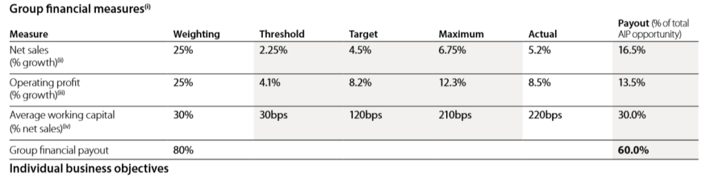
Source: Diageo 2018 AR, p. 81.
This looks absolutely good. Growth and capital tie-up are included into the performance measures. But wait, there is a footnote to the “Average working capital” measure. What does it say?
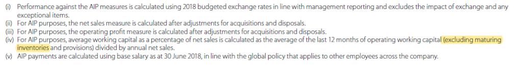
Source: Diageo 2018 AR, p. 81, own emphasis.
If you cannot read it – it is written in very small letters – here it is again:
“(iv) For AIP purposes, average working capital as a percentage of net sales is calculated as the average of the last 12 months of operating working capital (excluding maturing inventories and provisions) divided by annual net sales.”( Diageo 2018 AR, p. 81, again own emphasis.)
Take this: Maturing inventory is excluded from the working capital measure! This means, management perfectly benefits in its annual bonus from the above-shown transformation effects on revenue and profit growth but it does not have to pay the price for the increasing capital tie-up. We can see in the above analysis on our hypothetical case (‘Development of inventory total vs. non-maturing only’) how much the different working capital measures differ. And we highlighted clearly how important the inclusion of the capital tie-up is to get the whole picture.
Diageo management, however, here gets paid for growth out of nowhere! It is a clear confrontation with the basic idea of the switching business model, and it does not make a lot of sense for the case of a company that increases the proportion of maturing inventory over time. It rather incentivises management to go for more and more maturing inventory – whatever the fair value development of these maturing products is over time, so even if the fair value appreciation is for some products lower than the cost of capital (which would mean an equity value destruction). This is not a proper incentive at all.
If we look at the other years we can see a similar picture – but with one interesting twist. We first reproduce our graph from above (growth in maturing inventory of Diageo) but with additional information on how Diageo deals with the maturing inventory business in its capital efficiency measure of the annual incentive plan.

Source: Diageo ARs, legend: WC means that Diageo uses a working capital efficiency measure (working capital divided by sales) in the particular year, CC means that it uses a cash conversion measure, and FCF means that it uses a free cash flow measure. YES means that maturing inventory is excluded, NO means that it is not excluded.
We can see that since 2014 Diageo kicks-out the capital tie-up effects of maturing inventory from its short-term management remuneration scheme. It is not a big economic difference whether the company uses cash conversion of working capital measures (albeit with some minor quantitative changes). But it is quite interesting that Diageo started with the exclusion of maturing inventory exactly in the year where the recorded the biggest relative increase in this position, i.e. where capital tie-up measures are punished the most (on an un-excluded basis).
To be fair, it might be that the additional revenue and profit growth is already included somehow in the thresholds of the efficiency benchmarks (although we have to say that the switching strategy entails an automatic inventory/sales ratio improvement over time if one excludes maturing inventory here). And that the management gets still fairly remunerated based on the set thresholds and targets. We simply do not know enough about the concrete ideas behind this remuneration system. But the structure of the incentive measures is very weak. In this concrete case of the Diageo business model one could clearly set up a much more powerful incentive scheme (e.g. by simply including maturing inventory into the working capital measure) to align shareholders’ and management’s goals.
Summary: Investors are well advised to dig deeper into the periodical value accretion of the maturing liquors of Diageo. This is the real critical point behind the Diageo strategy. How much has to be invested initially, how much do they earn from it? Anyway, gross profits and profit growth is for this business not comparable with other companies who do not run such a relevant maturing liquor inventory business. And the structure of the remuneration scheme is simply inappropriate for this business model.
Disclaimer: As always, we hold no economic stake in the company involved in this blog post – in whatsoever direction. We base our analysis on imperfect information and hence we might be wrong with some conclusions. This is just our subjective view and no investment recommendation at all.