Dealing with stock options (employee stock options ESOs or employee stock option programs ESOPs) in business valuation is not easy. A proper treatment of these instruments is particularly tricky if the options are structured with specific contingent exercise features which makes the concrete valuation of single options quite challenging. The general technique of the consideration of such programs as part of a DCF-valuation is, however, rather straightforward. This is the topic of today’s blog post where we analyse this aspect by way of a simple example with plain-vanilla stock options.
Starting point is a company that is (for reasons of simplicity) fully equity-financed and earns a net cash flow (= earnings) of 100 Euros p.a. – paid at the end of the period and expected stable until eternity. The cost of equity of this company is 10%. The company has 500 shares outstanding. We are currently at the beginning of period 1. Taxes are ignored.
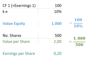
In this situation where no stock options are outstanding the value per share can easily be calculated as 2.00 Euros. Earnings per share are 100/500=0.20 Euros.
Now let’s imagine that the company switches from top-management cash-salary payment to a partial remuneration via equity-settled stock options for the current period (i.e. period 1) only. More precisely the company substitutes 75 Euros of cash compensation by giving out stock options worth 75 Euros (50 options at a strike of 2.00 Euros which have a fair value of 1.50 Euros each due to the time value). Here it is important that for reasons of comparability the company does not give any extra-grants to management but just switches from one way of paying a remuneration to another one.
Now a couple of things change. First, the cash flows increase in this particular period 1 (75 Euros less cash pay-out). However, the earnings stay at the level of 100 Euros as the 75 Euros ESOP value are expensed (since the introduction of IFRS 2 resp. SFAS 123 in 2003 resp. 2004 the fair value of ESOPs granted in a particular period have to be expensed in the P&L over the vesting period [here immediate vesting is assumed]).
Second, from the viewpoint of shareholders (not from the viewpoint of the company) a liability of 75 Euros is built-up. This is the case as at the time of giving out the options (here: end of period 1) the economic situation of outstanding options can only be reversed – or cancelled – by paying 75 Euros to the beneficiaries of the options.
Third, while the value per share is still calculated the normal way, the calculation of earnings per share (EPS) requires some more clarification. The relevant EPS in case of the existence of instruments outstanding that can be converted into equity is the so called diluted EPS. According to IAS 33.31, diluted EPS is calculated not only by adjusting the earnings according to IFRS 2 but also the number of shares for the effects of dilutive options and other dilutive potential ordinary shares (the effects of anti-dilutive potential ordinary shares are, however, ignored in calculating diluted EPS, IAS 33.41).
Furthermore, in calculating diluted EPS it is assumed that outstanding dilutive options and warrants are exercised. The assumed proceeds from exercise, i.e. the strike times number of options, should then be regarded as having been used to repurchase ordinary shares at the average market price during the period. The difference between the number of ordinary shares assumed issued on exercise and the number of ordinary shares assumed repurchased shall be treated as an issue of ordinary shares for no consideration, i.e. as a net increase of the number of shares [IAS 33.45]. This is called the treasury stock method.
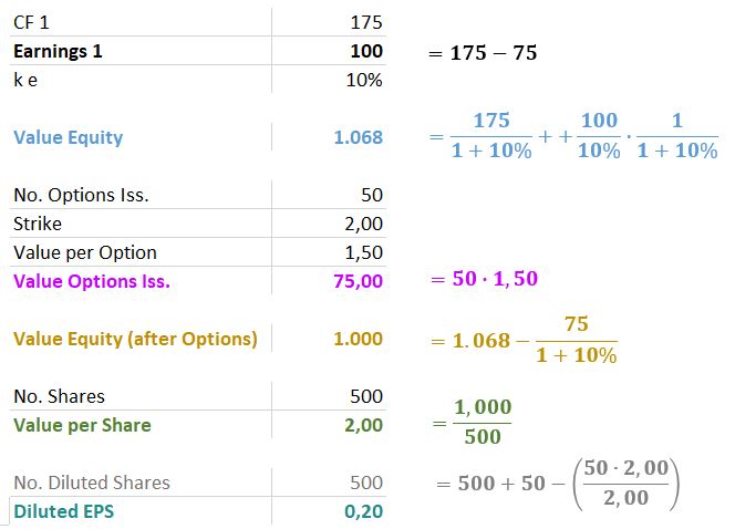
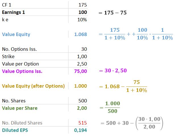
In the concrete example where options are given out with a strike equalling the current share price the diluted number of shares does not change, and hence the diluted EPS do not change, either. However, if the 75 Euros stock option compensation is rather the result of an issue of 30 Stock options at a fair value of 2.50 Euros each (with a strike of 1.00 Euro, i.e. in-the-money at time of issuance) then things change. As now the proceeds that can be used to repurchase ordinary shares according to the treasury stock method are lower, the diluted number of shares is higher.
If now the company plans to issue stock options worth 75 Euros (and perfectly substituting a part of the cash salary to management) in every period, then the following table is the result. We can see that nothing changes in terms of present value or EPS for period 1. This is an important finding: future stock option issuances are value neutral as long as they take place on a fair basis, i.e. perfectly substituting other cash expenses.
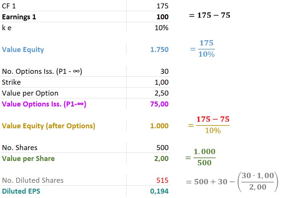
This table also highlights another important aspect. When considering future expected stock option issuances it is possible to go the split-way shown above (higher periodical cash flows + consideration of a future ‘option liability’) OR to do the short-cut by taking the fair value of options issued in every period as a cash-flow-like component and directly deduct it in the cash flow forecasts. I.e. the “Value Equity (after Options)” can also be calculated by:
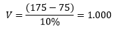
As the second variant is much easier to operationalise it is recommended to go this way.
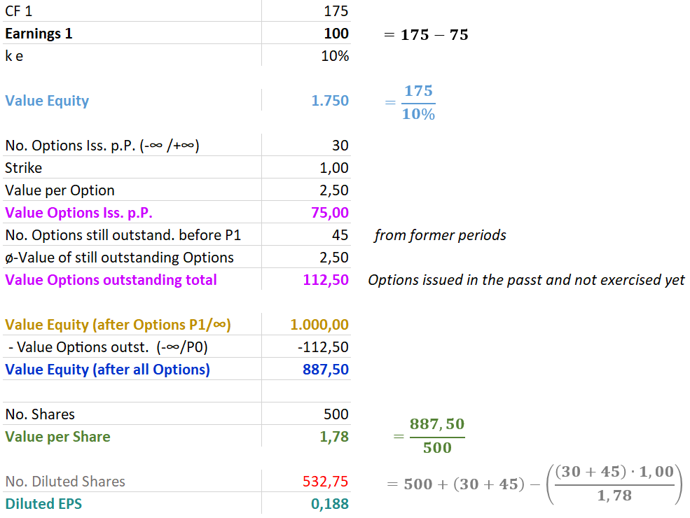
Finally, it is considered that not only options are granted in the future but that there are also options that have been granted in the past (and not yet exercised). In our example, there are assumingly still 45 options outstanding from former periods, at a strike of 1.00 Euro each and a current fair value of 2.50 Euros each. These existing options can no longer be seen as a compensation for cash salary payments now (even if they have been in the period of granting) as they are still an existing claim to the equity of the company although the services (work of top-management) has already taken place in the past. This is why they have to be treated – from the viewpoint of time of valuation, i.e. beginning of period 1 – as naked liabilities at fair value.
This changes the value of equity (after options) and the diluted EPS.
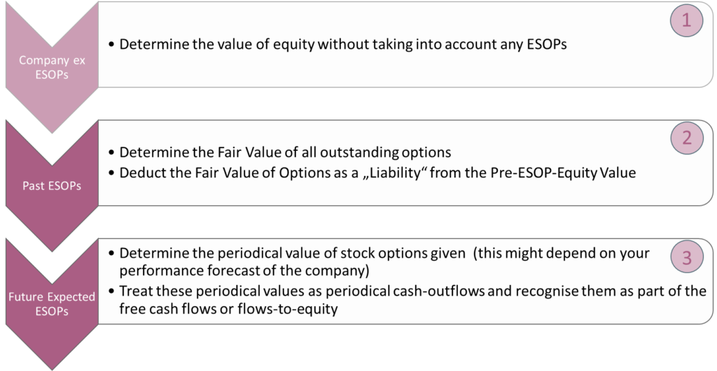
With these findings we can now set up a ‘best practice’ for considering stock options in DCF-valuations – at least for plain vanilla programs.
In one of our next blog posts we are going to have a deeper look at some of the specificities of stock option programs.