Crises are times of change and of uncertainty. For equity investors this requires some fresh thinking on fundamental analysis (see HERE and HERE) but also some fresh approaches to the determination of the cost of capital of companies. The latter one is the topic of today’s post. In our discussions we will focus on the WACC/CAPM environment as this is an often used framework for investors. However, some of the comments can also be used for other cost of capital approaches.
The basic challenge with the cost of capital during crises is that we often observe a structural break in one or more of our key structures for cost of capital determination. While in stable times we often rely on historical data for e.g. beta derivation or the determination of market risk premiums, this no longer works in crisis times as the recent past is no longer representative for the current situation and the future. As a consequence, we have to dare to go away a bit from our purely past-oriented approach and bring in some more forward looking ideas. Here we go:
- The Cost of Equity: Reading the CAPM from a stability/instability point of view!
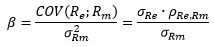
In most practical settings, the CAPM is depicted as follows (or similar):
![]()
With:
and
![]()
Here ke = cost of equity, Rf = risk free rate, Re = Equity rate of return of the target company, Rm = Equity Market Return, MRP = Market Risk Premium, σ = standard deviation, ρ = correlation coefficient and COV = Covariance.
During crises, the problem is that all components of the CAPM risk premium change:
(1) Beta is no longer the same as there are new correlations with the market (this can be nicely observed currently for many businesses in the retail sector [both consumer staples and discretionary], depending on the concrete business model into different directions] and also as there are new idiosyncratic risks to the single business models, i.e. mostly higher volatility of the rates of returns, as well as also higher market volatilities. One important point is here: we cannot say in which direction betas change without any deeper fundamental analysis. The direction clearly depends on whether market exposure of the business model increases or decreases, and on whether the increased volatility of the business is now higher or lower than the increased volatility of the market.
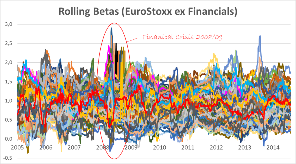
The following graph shows the development of 100-day/daily-Betas (unlevered) of the enlarged Eurostoxx index (ex-Financials) between 2005 and 2015. We can at least qualitatively see here that betas are not at all stable over time in general (something that is worth some thoughts on practical applicability of the CAPM already in stable times) but – most importantly – that the financial crisis 2008/2009 was a real big time of extreme beta values.
But not only the range of betas was extreme during the financial crisis. If we look closer at this period we can see that the volatility of single betas was also very high for longer. This can be seen in the following graph which shows the average 15-day standard deviations of betas during 2005 to 2015. Taking these two observations together, we can see that the financial crisis really was a period of change for betas, and a break with historical patterns.
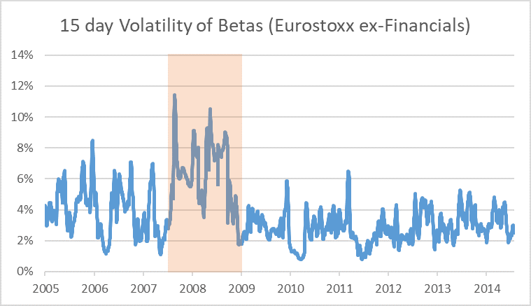
If we look closer at the development of betas over time after the financial crisis we can see some trend of reversion towards the mean, i.e. some normalisation over time (which is also in line with earlier academic findings, see e.g. Blume (1971), On the assessment of risk, Journal of Finance, No 1, p. 1-10, and Blume (1975), Betas and their regression tendencies, Journal of Finance, No 3, p. 785-795). However, this normalisation takes quite a lot of time for some stocks.
(2) The market risk premium is also changing, or more precisely: increasing. In times of crisis, the general uncertainty increases and hence also the premium that investors require for bearing this higher uncertainty. In the following graph, we show the results of our implied market risk premium model over the last years. As such implied models are highly assumption-driven we also show the upper and lower range limits (grey) of our measures. The model shown here is a proprietary one that makes use of some subjective adjustments in order to overcome the data quality problems (timeliness and long-term projections) that we usually have when applying implied-cost-of-capital models. But we do not want to go too deep into the details of calculation here, and the concrete application is not of super-high relevance for this post. Anyway, for some background information on such models in general, see e.g. Damodaran (2019), Equity Risk Premiums (ERP): Determinants, Estimation and Implications – The 2019 Edition, p. 74 ff.
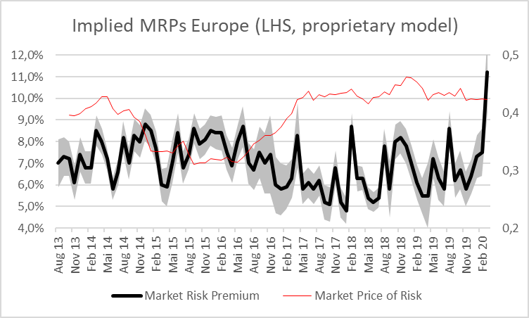
We can see here the steep increase in March 2020 to a value of the market risk premium of 11.20% according to our model. Admittedly, March 2020 has seen quite a big range of implied market risk premiums due to the huge volatility of stock prices and the big investors‘ mood swings. The 11.20% are the average value for the month so far.
As both variables, Beta and MRP, change in times of crisis it might be a good idea to split these two variables further (or at least to split the risk premium in a different way) so that we can separate the parts of the CAPM risk premium that change from the ones that stay – more or less – stable. This should allow us to apply our forward looking analysis in a more focused way. So let’s go! From the information on the CAPM formula above we know:
![]()
Now the risk premium is split into a target company specific part (σRe ∙ ρRe,Rm), and a market related part – (Rm-Rf)/ σRm. Interestingly, this market related part equals the Sharpe-Ratio for the whole market. We call it here the “market price of risk”. It is the premium that investors require for taking one unit of risk. (Comment: we know that in academic literature the market price of risk is calculated by dividing the market risk premium by the variance of the market returns and not by the standard deviation of the market returns, but for fundamental analytical reasons it makes more sense to define the market price of risk as we do it here in this blog post).
In the graph above (“Implied MRPs Europe”) we can see the market price of risk, i.e. the market Sharpe ratio, depicted as a red line. It shows characteristics of relative stability over time, at least for certain time periods or regimes. Attention: The market price of risk is calculated here using our implied market risk premiums and forward looking volatility estimates based on the VStoxx-index, so it is still a forward looking measure. Depending on the model used for deriving market risk premiums the results might differ from ones shown here.
With the risk free rate seen as externally given here, it is worth to have a look at the remaining parameter of the market-price-of-risk formula, the volatility σRm. We do this below by looking at the timely development of three international volatility indices, the VIX, the VSToxx and the VDax.
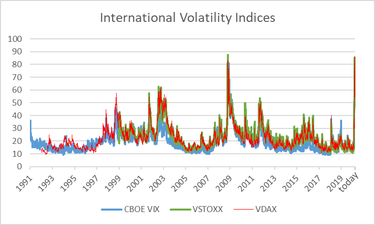
These indices use forward looking volatility measures (i.e. derived from the pricing of equity option contracts). This means they present a very timely measure of volatility of markets. From the graph we can see the massive increase in volatility (close to the peaks seen during the financial crisis 2008/2009) during the last days.
- What does this mean for the derivation of the cost of equity?
While there is certainly no silver bullet for determining the cost of equity in such an environment, we think it is at least worth to apply the CAPM stability/instability approach as a plausibility check when determining the cost of equity. This means:
- Market risk premiums usually increase in times of crisis. However, historical market risk premium models are not flexible enough to deal with the sudden change in the market environment of the coronavirus crisis. And many forward-looking market risk premium models need too much time in order to show more or less proper results (mainly due to slow adjustment processes for sell-side analyst estimates that are used as an input). A component that is rather stable, however, is the market price of risk, i.e. the premium investors require per unit of risk. Although admitting that this parameter shows regime change effects as well, we can treat it as a constant variable here in a first step.
- If we split the CAPM risk premium into a) the market price of risk, and b) the company specific part (σRe ∙ ρRe,Rm) then we can approach this second term at least partly from a fundamental point of view: How have correlations of the target company’s business model with the overall market changed? What is the volatility of the equity rate of return of the target company (something we can also approach via implied option volatilities [from comparable companies])? Not easy to answer, but due to a lack of usefulness of historical information such a partly fundamental approach is definitely kind of necessary here.
- In sum: Applying the stability/instability approach we have NOT determined the market risk premium per se, NOR have we determined the beta. But we have determined β∙MRP altogether. And this also gets us to the point. Take care: There are definitely also strong assumptions and weaknesses to this approach, so it is not the one and only solution to derive the cost of equity in this environment, but at least it offers us a new perspective on this high-uncertainty valuation problem. And new perspectives are (at least as a plausibility check) a very welcome help in this current environment.
- Can’t we just keep our cost of equity at the same level as before?
I got often asked why one should do all this adjustments if both beta and the MRP will go back to old levels some day in the future. Isn’t it possible to simply ignore this more or less short phase of parameter distortion in our valuation models?
The answer is a clear: No! Without going too deep here, the parameter movements in times of crisis are highly material (as are the value changes in times of crisis). While there might be some effects that we can observe at capital markets currently that are not fundamentally driven (i.e. the price changes due to market microstructure, liquidity-triggered trading of some investors, etc.) most of them are clearly fundamental. They are the result of new projections on the performance of companies and of the increased uncertainty about the concrete outcome of these projections.
Clearly, if our models show us an implied market risk premium of 11.20% these days, then this is not only a one-period risk premium. It is rather the average market risk premium over the whole discounting period (i.e. until eternity).
And, finally, while we also expect that one day equity parameters on average will find back to their long-term value, this does not mean anything for single businesses. And business valuation is clearly about single businesses. Averages do not help us at all here. The famous Oaktree Capital founder Howard Marks described this point nicely in the context of insolvency risks: “Never forget the six-foot-tall man who drowned crossing the stream that was five feet deep on average. It’s not sufficient … to survive on average. We have to survive on the bad days.” There is nothing to add from our side in terms of why it is necessary to bring your valuation parameters always up to date.